let’s talk a little bit about the basics of Hadoop where it came from what it’s for what it’s all about. All right let’s dive right in and talk about the Hadoop ecosystem. The mascot is this yellow elephant here and we’ll talk about why in a minute.

WHAT IS HADOOP?

let’s talk a little bit about the basics of Hadoop where it came from what it’s for what it’s all about. All right let’s dive right in and talk about the Hadoop ecosystem. The mascot is this yellow elephant here and we’ll talk about why in a minute.

A. Definition

“An open source software platform for distributed storage¹ and distributed processing² of very large data sets on computer clusters built from commodity hardware³” – Hortonworks (one of the major vendors of Hadoop platform)

1. Distributed storage is one of the main feature that Hadoop provides the idea is that you are not going to be limited by single hard drive. As if you’re dealing with Terabytes of information (big data) or even more its very difficult to store all of it in a single physical hard drive. The advantage of distributed storage is that you can scale horizontally i.e. you can add more nodes(computers) to your cluster and their hard drive will become part of your data storage for your big data. What Hadoop gives you is the way of viewing all of the data distributed across nodes and one single file system. And not only that its also very redundant so if one of those machines happens to bust into flames and melt into gooey puddle of silicon! Hadoop can handle that by keeping backup copies of your data in other places in your cluster and it can automatically recover and make your data very resilient and reliable.

2. It gives you is distributed processing so not only can it store vast amounts of data across an entire cluster of computers it can distribute the processing of that data as well. whether you need to transform(map) all that data into some other format or to some other system or aggregate(reduce) that data in some way Hadoop provides the means for actually doing that all in a parallel manner so it can actually utilize all the CPU cores on your entire cluster and solving that problem in parallel. And that way you can actually get through all that data very very quickly. So you know you don’t have to sit there with a single CPU chugging away on a petabyte of information. It can divide and conquer that problem across all the PCs in a cluster.

3. By commodity hardware we don’t mean cheap we just mean readily available and general purpose machine that you can rent from say Amazon Web Services or Google or any of the other vendors out there that sell cloud services. You can just keep on adding as many computers as you need to handle the amount of data you have.

B. Hadoop History

Hadoop wasn’t the first solution to big data problem. Quite honestly Google is the grandfather of all this stuff, so back in 2003 and 2004 Google published a couple of papers about how they were handling things internally. Google published papers about there distributed file system Google file system (GFS) and processing engine MapReduce. So GFS is basically what inspired Hadoop Distributed File System (HDFS) and MapReduce is what inspired Hadoop’s distributed processing, and in fact they didn’t even change the name, Hadoop processing engine is still called MapReduce. Hadoop was developed originally at Yahoo when Doug Cutting and Tom White started putting Hadoop together in 2006. Story goes that Hadoop was actually the name of Doug Cutting’s kid’s toy Elephant. And apparently this is the actual yellow stuffed elephant named Hadoop that the project was named after. So now you know why Hadoop’s mascot is a yellow elephant. [reference -> https://www.youtube.com/watch?v=irK7xHUmkUA]

Fig: Twitter Link

HADOOP ECOSYSTEM

There’s a lot of different ways of organizing these systems and the following is just what makes sense to me. Also there are a lot of complex interdependencies between these systems so there’s really no right way to represent these relationships.

We can split things up here into two general areas here: the core Hadoop ecosystem which consists of the frameworks that ships directly with Hadoop i.e. HDFS, Yarn and MapReduce and other ancillary systems, these are sort of add on projects that have come out over time that integrate with Hadoop and solves specific problems.

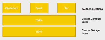
Fig: Hadoop Simplified Architecture

i. Cluster Storage Layer - HDFS (Hadoop Distributed File System)

So let’s start at the base of it all which is HDFS that stands for the Hadoop distributed file system. Remember we talked about Google File System (GFS). HDFS is the Hadoop version of that and is the system that allows us to distribute the storage of big data across our cluster of computers so it makes all of the hard drives on our cluster look like one giant file system.

Handling big files

It can handle massive data and it does this by breaking up those files into blocks and those blocks are actually pretty large it’s 128 megabytes by default (which is configurable) so you know we’re talking about big files here. By splitting up these large files into blocks we’re not limited by the storage limitations of a single harddrive. It allows you to distribute the processing of one of these large files so if we split that large file up across several different computers that means different computers can access different parts of that data and process it in parallel. Also those blocks can be stored across several commodity computers and it doesn’t just store one copy of each block. In order to handle failure. it will actually store more than one copy of each block and so that way if one of these individual computers goes down HDFS can deal with that and actually start retrieving information from a different computer that had a backup copy of that block and it can do this in a clever way such that if a single node goes down you don’t actually lose any blocks from any given file because there’ll be another block stored somewhere else at all times. The key point here is that it allows you to purchase commodity computers you don’t have to get a special special purpose expensive computers that have high availability because as the the side effect of this architecture is that if a single computer goes down it’s not a big deal. We can just fail over to another node that has a copy of that block somewhere else.

HDFS Architecture

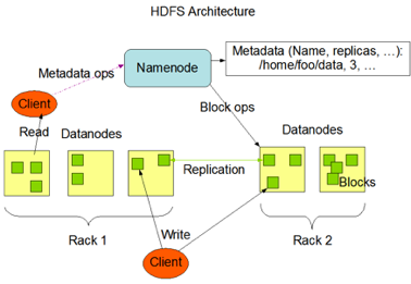
Fig: HDFS Architecture [reference -> https://hadoop.apache.org/docs/r1.2.1/hdfs_design.html]

**Now, the above figure explains HDFS Architecture and this looks pretty complex, right?**

Let us break this Architecture model into smaller process and try to understand the following.

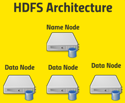
Fig: General Architecture

Let’s see about how HDFS architecture works and in a little bit more depth here. There is a single name node and this name node is what keeps track of where all data blocks live (metadata) through FsImage. So basically it’s maintaining a big old table of a given file name under some directory structure and it knows where to go to actually find every copy of every block that’s associated with that file.

EditLogs: Also it’s also maintaining what’s called an edit log that maintains a record of what’s being created, modified and stored so that it can keep track of where everything is as things get moved around or new files get created. So that name node is what keeps track of what’s on all the data nodes and individual data nodes are ultimately what your client application will be talking to. Once it queries the name node to figure out where to go to for a given bits of information and the data nodes are what actually store each block of each file. And they actually talk to each other as well to maintain those copies and replication of those blocks.

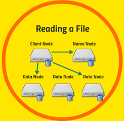
Fig: Reading File from HDFS

Let’s take a closer look at the example of reading a file in HDFS. So let’s say you have an application running on some client that needs to access data stored on the HDFS. First thing it will do is talk to the name node and say “hey I want to get this file” and the name node will come back and say “OK your file lives on these blocks on data nodes one and three” (The Namenode responds with number of blocks, their location, replicas and other details) and then your client application will know that it needs to go back to data node one and data node three to retrieve the blocks that it need for this particular file.

Now your high level application (spark, MapReduce etc.) won’t actually be dealing with it at that level. There are low level client libraries that will be used and it’s all happening under the hood, but architecturally your client would first talk to the name node to figure out where that file is stored which blocks are on which data nodes and which ones are the most efficient data nodes for you to reach from your client and it will then direct your client to go retrieve data directly from those data nodes that it wants.

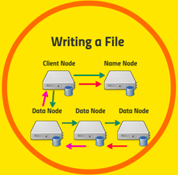
Fig: Writing File to HDFS

What if we’re writing a file? It’s a little bit more complicated.

So let’s say my client application wants to create a new file on HDFS. First the client is going to approach the Namenode and Namenode will create a new entry in the FsImage and EditLogs. The Namenode responds with a number of blocks, their location, replicas and other details. Based on information from Namenode, client split files into multiple blocks. After that, it starts sending them to first Datanode. Now let us assume that there are three Datanodes and Datanode 1 and 2 are on same Rack and Datanode 3 is on separate Rack. The client first sends block A to Datanode 1 with other two Datanodes details. When Datanode 1 receives block A from the client, Datanode 1 copy same block to Datanode 2 of the same rack. As both the Datanodes are in the same rack so block transfer via rack switch. Now Datanode 2 copies the same block to Datanode 3. As both the Datanodes are in different racks so block transfer via an out-of-rack switch. When Datanode receives the blocks from the client, it sends write confirmation to Namenode. The same process is repeated for each block o the file [reference -> https://data-flair.training/blogs/hadoop-hdfs-architecture/].

ii. Cluster Data Warehouse (HBase)

Let’s talk about HBase. HBase is actually built on top of HDFS. So if you’re storing massive datasets on an HDFS file system, HBase can be used to actually vend that to the outside world at a very large scale.

Note: understanding of CAP theorm helps with Data Warehouse selection.

CAP Theorem:

Whenever we are working with distributed systems, which is usually the case in big-data environment we need to consider cap theorem and architect according to the requirements. Most of the data warehouse technologies handling big data are mpp (Massively Parallel Processing Database) henceforth are distributed. So we should understand CAP Theorem and select data warehouse accordingly.

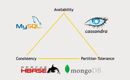
CAP is an acronym for Consistency - Availability - Partition Tolerence.

CAP Theorem states that we can only maintain two out of three: consistency, availability, or partition tolerance in a distributed system. So again, the way to think about this is when you’re thinking about the scale of your requirements, do you need to have partition tolerance? Do you have sufficient scale, where you know you’re going to eventually need more than one server serving up the data just for handling the transactions you’re talking about, and also for the scale of the data that you’re talking about? If so, partition tolerance is non-negotiable, you need that one, and your only real choice in that case is consistency or availability. And that will determine which one of these sides of the triangle you might want to lean toward.

So the type of application will determine what you want there.

Only you know the actual requirements that you have for availability. Is it actually OK if your system goes down for a few seconds or a few minutes? If not, then availability’s going to be your prime concern.

Is it OK if you have eventual consistency, where, if you write something, people might get the old value back on subsequent reads for a few seconds? If so, who cares about consistency, right? Again, I would take availability instead. But if you’re dealing with something that’s dealing with real transactional information like, you know, stock transactions or some sort of financial transactions, you might value consistency above all else, and in that case, you want to really focus on that corner of the triangle.

So again, understand how to read this diagram here. Cassandra, for example, lies on the availability and partition tolerance side of the triangle, where we’re favoring these two over consistency. And when we talk about HBase and MongoDB, they’re favoring consistency and partition tolerance above availability. Now, I should point out that the CAP theorem isn’t really a hard-and-fast rule.

The **reality** is these tradeoffs have become a little bit more loose in recent years. so, for example, consider Cassandra: is it really trading off consistency for availability and partition tolerance? Well, you can actually configure the amount of consistency that you want from Cassandra - you can tell it, “I want to make sure I get back the same result from every replica of this data before I actually consider that transaction to be final”, and if you’re running it in that mode, you’re kind of getting all three to some extent.

Even with MySQL, for example, you can set up sharding and make it partition-tolerant, but it’s just more of a hassle and more of an administrative problem. And, above all, my advice is always to keep it simple, so, you know, if you don’t need to set up a highly complex NoSQL cluster and something that needs a lot of maintenance, like, you know, MongoDB or HBase, where you have all these external servers that maintain its configuration, don’t do it, if you don’t need to. Think about the minimum requirements that you need for your system and keep it as simple as possible.

HBase Architecture:

So what is HBase? It is a non-relational scalable database built on HDFS, which we already said. So, just like every other NoSQL solution, it does not have a query language, but it does have an API that can very quickly answer the question “what are the values for this key?” or “store this value for this key”. And it’s built on the ideas behind Google’s BigTable database. Papers that were published by Google about 10 years ago, where they had the problem of storing information about links to all the web pages on the entire planet, which, obviously, is a big-data problem, and they developed something called BigTable to solve that problem. Now, HBase is just pretty much a straight up implementation of BigTable, where they just changed some of the names, so it’s an open-source implementation of the algorithms and systems described in BigTable. HBase doesn’t really have a query language, there’s no, like, equivalent of SQL that you can do on it. All it has is an API, so it can do what we call CRUD operations. CRUD stands for “create, read, update, and delete”. So it offers transactional access to you: creating a row in a database, reading back the values of a row in a database, updating a row in a database, or deleting a row in a database. That’s about all it does, but it does it really, really quickly and at a very large scale. That’s the power of HBase. Take a look at its architecture here.

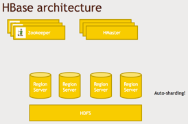
Fig: HBase Architecture

So this is how HBase works under the hood. Basically, it’s split up into different region servers. And when we talk about regions, we’re not talking about geographic regions, we’re talking about ranges of keys, so it’s just like sharding or range partitioning in more traditional database systems. But the magic of it all is that it can automatically adapt, so, as your data grows, it can automatically repartition data, and if you add more servers to the mix, it can automatically deal with that at runtime. Auto-sharding is a very complex mechanism that involves write-ahead commit logs and, merging things together over time asynchronously.But you don’t have to worry about those details - HBase does it for you. So all you need to know is that it can automatically distribute your data amongst a fleet of region servers, And these are all sitting on top of your HDFS file system, which itself is distributed, right? So you can have HDFS hosting very large files(HFIles) across an entire cluster of computers that are broken up into blocks, and again, some of what HBase gives you is taking all these little tiny records that are in your individual rows and clopping them together into larger files which are better managed by HDFS. So again, it’s all transparent to you.

Now, when you have an application that’s actually talking to HBase - a web application or a web server - it’s not actually going to talk to master nodes (HMaster) directly, it’s going to be talking to region servers directly, but these master servers (HMaster) keeps track of the actual schema of your data, where things are actually stored, how they’re partitioned. HMaster doesn’t have to get queried very often, so it’s not really going to be a bottleneck, but it is sort of the mastermind of your HBase cluster that knows where everything is, and that, in turn, depends on the technology called ZooKeeper. So it’s a highly available system that can keep track of who the current master server is for your HBase instance. And if one master goes down, ZooKeeper can keep track of who to go to next and tell everyone about who the master is.

Note: So at a high level. You know, the key here, though which data is partitioned amongst different region servers: there are master servers (HMaster) that keep track of where everything is, and the data itself is actually stored on big files (HFiles) on HDFS.

HBase’s data model:

Like with any database, it’s going to have this concept of rows, where each row is identified by some unique key value. So, for example, you might have a database of customer information, where the rows are identified by a unique customer ID key. If you’re coming from the relational database world, you know that will be the primary key, and each row contains information associated with that key. So, for example, a “customer” table might have rows identified by a customer ID, and it might have columns that map to the customer’s first name, last name, address, zip code. Now, what’s different about HBase is that it has the concept of column families. So you don’t define a fixed set of columns for each row in your database. Instead you define column families, and each column family can contain a very large number of individual columns. This comes in handy where you have cases of sparse data. You know, for example, let’s say you have a database of movie ratings broken up by each user. You don’t want to have to actually store a column for every single movie that was ever created to hold the ratings each user has for each movie. What you can do instead is create a column family for ratings as a whole and then have a large number of columns that map to each individual movie. But it’s OK if each customer doesn’t have data for every movie. You know, the power of HBase is that it can deal with sparse data like this, so it doesn’t actually consume any space to have a column that’s missing data. So the model that you should want to think about with HBase is how can I have a very small number of column families associated with each row of my database, but then I can actually blow up each column family potentially into a large number of columns. And you don’t have to, either. You can have a one-to-one mapping as well, so you can have a column family that’s just “customer name” and leave it at that. And that’s going to be your column, you know, but you do have that power splitting up a column family into potentially a very large number of columns, which may be populated in a sparse manner. Now, we also have the concept of a cell that’s given by the intersection of a row and a column, and another cool thing about HBase is that it can have many versions of each cell, so it can actually store a history for each cell in your database table, and it can do that automatically based on timestamps. You can actually say, “store all the information that was given within the last week for this given row-column intersection”. And you can also just say, “retain this many versions of a given cell”. So, for example, you know, “keep the last three values that I saw for this particular piece of data”.

It makes more sense when we look at an example, So let’s do that. Let’s look at the problem that Google actually was trying to solve with BigTable, which became HBase.

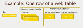
Fig: HBase Data-Model Example

They wanted to be able to track all the links that connect to a given web page. So, let’s say they’re trying to figure out who links back to CNN.com. This is what their schema might look like in BigTable, or HBase in our example. And this comes straight out of the BigTable paper, so they might have a key that is a web page or a web site, and they actually store this in reverse order. So instead of www.CNN.com, they do it backwards in com.CNN.www. The reason is that keys are stored lexicographically within HBase. So if you’re trying to minimize disk seeks and you know that you might want to have, you know, web pages on the same web server, you might want to use something like this. Sometimes you’ll see like, you know, www.CNN.com, or si.CNN.com, there might be variations on www, and you want those all to be together within the database, so that’s why they do things like that. And what do their actual columns look like? So they’ve set things up into a couple of column families in this example. One is the “Contents” column family, and there’s only one column within this column family - “Contents” itself. But you can see they’re using the versioning feature to actually keep three copies of the contents of this page. So they’re actually scraping CNN.com and storing the last three incarnations of that page that they came across, the last three crawls. who knows what they’re really doing under the hood today, but this is what they’re describing in the paper. And then what they have is an “Anchor” column family. So this is where they’re storing all of the pages on the web that link back to CNN.com. The syntax for describing a column in HBase is :, so "Anchor:cnnsi.com" would represent a link from cnnsi.com and anchor. So, for example, someone put the word CNN on a web page, on cnnsi.com, linked the word CNN back to CNN.com, that link text is what actually gets stored as the column value. And, as another example, let's say a web site called my.look.ca actually also linked back to CNN, but they actually linked the word CNN.com. You don't want to have to store the fact that CNN.com is not linked to by five million other web sites, right? You just want to be able to store the actual web sites that do link back to it. So that's the power of this particular data model.

Interacting with HBase:

There are many ways to access HBase, one is through an interactive shell, so if you’re actually logged into the server that HBase is running on, you can type in “HBase shell” and interactively create commands to create new tables, you know, create the column families in that table and so on and so forth, or drop tables, do whatever sort of maintenance you need to do. But for runtime, you know, to actually use the power of HBase, you’re usually going to be accessing it from, you know, some service(connector) of some sort. So you’re going to have some web server that’s trying to put together a web page based on this data or something. So, at its lowest level, there’s a Java API for Hbase, because HBase is itself written in Java, and if you have a Java-based web server or application, then you can talk to that directly. There are also wrappers available for other languages, like Python and Scala, for example. There are also connectors available between Hbase and things like Spark, Hive and Pig.

iii. Cluster Compute Layer (YARN)

What is YARN?

YARN stands for Yet Another Resource Negotiator, and it was introduced in Hadoop version 2 and the idea there was actually split out the problem of managing the resources on your cluster from MapReduce itself. So in Hadoop 1 MapReduce was this monolithic framework where, you know, you ran mappers and reducers and the resource negotiation(YARN) was just part of it, but with YARN they split out the resource negotiation part which allowed the development of MapReduce alternatives such as Spark and it turns out Spark using directed acyclic graphs can outperform MapReduce quite a bit, so that really does unleash a whole world of new possibilities and new performance that we couldn’t have gotten otherwise. So, thank you Hadoop people for splitting that out!

Where does YARN fit in architecturally? Well, at the bottom of our stack here on Hadoop we have HDFS, which is the cluster storage layer, the Hadoop distributed file system, so if you recall, that’s just the system that allows us to spread out the storage of big data across your cluster by breaking it up into blocks that are replicated across the various nodes in your cluster. Now, YARN sits on top of that storage layer, so YARN is the compute layer for your cluster and it can execute specific jobs or tasks or, you know, application chunks basically, if you will, that are depending on processing certain chunks of data that’s on your HDFS cluster. So the whole idea of YARN is to split up the actual computation across your cluster whereas HDFS is splitting up the data storage across your cluster, and these two are pretty tightly integrated actually because YARN tries to maintain data locality. If you try to execute a job that is specifically looking to operate on some specific blocks of data in HDFS, YARN will try to align those on the same actual physical host as much as possible.

So YARN is basically what’s managing the computing resources of your cluster and each HDFS is what’s managing the storage resources of your cluster. On top of YARN we can write different applications such as MapReduce, such as Spark and such as Tez and these are YARN applications that sit on top of the compute layer which in turn sits on top of the storage layer.

How do YARN Works?

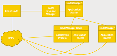
You kick off an application from your client, a YARN resource manager will then kick off an application master that runs on whatever node has capacity to run it, and then that application master is responsible for working with YARN to spin up more nodes that have their own NodeManagers that run specific application processes. So that’s all YARN is doing, is trying to make sure, it’s trying to figure out where to run all these application processes, where to split up these nodes and how to evenly distribute the processing of that information across your cluster and do it in such a way that it minimizes data getting shuffled around your network, so, it’s both trying to optimize the usage of your cluster from, such as: CPU cycles and also trying to maintain data locality to ensure that a specific application process has as quick access as possible to the data blocks that it needs from HDFS. Your application (Client Node) talks to a resource manager to distribute the work to your cluster and in a high availability Hadoop environment there may be multiple resource managers that use ZooKeeper to keep track of who the main master is at the given point. So just because you see a single resource manager in that diagram does not mean it’s a single point of failure, there is a way to actually have redundancy there as well. We talked about data locality and there are also different scheduling options you can specify when you’re writing applications on top of YARN and these are usually configurable when you’re actually running an application.

YARN Scheduling

There are three types of schedulers in YARN are FIFO, capacity and fair.

• FIFO (which stands for First in First Out) just runs jobs in sequence, so if you request to run an application in YARN in FIFO mode and then you request a second application, the second application won’t start until the first one is finished, so it all just runs in sequence.
• Capacity means that if you’re trying to run multiple applications at once on your YARN cluster, they might run in parallel if there’s enough spare capacity, So if you’ve kicked off a MapReduce job, for example, on top of YARN that is only using a portion of your cluster, the capacity schedule can say “hey! I have some spare capacity here if someone else wants to run another application” that can run at the same time on the other nodes.
• Fair scheduler is a little bit different in that if you have a really big job running that is consuming everything on your cluster, but you try to get a small one and sneak it in, Fair might say “OK, I’m about to steal some resources back from this huge job just to give this small job a chance” because it’s not really going to make a big difference in the grand scheme of things.

So those are the different scheduling types you can configure with YARN, FIFO which just runs things in sequence which is nice and simple and easy to understand, Capacity which will make the best use of the capacity you have on your cluster and Fair which will actually try to give small jobs a chance even if a big one is hogging the entire cluster.

iv. Application Engine (SPARK)

What is Spark?

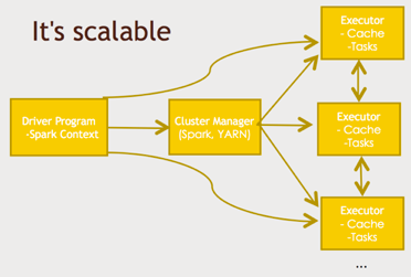
Well if you go to the official Spark Web site at spark.apache.org It will just say “A fast and general engine for large scale data processing”. Spark does give you a lot of flexibility where you can actually write real scripts using programming languages like Java, or Scala, or Python to do complex manipulations and transformations and analysis of your data and what sets it apart from other technologies like Pig for example is that it has a rich ecosystem that lets you do all sorts of complicated things like machine learning and data mining and graph analysis and streaming data that. Just like any Hadoop based technology Spark follows the same pattern where basically you have a driver program a little script that controls what’s going to happen in your job. And that goes through some sort of a cluster manager and you can use YARN that but that’s only one option like Spark can run on Hadoop but it doesn’t have to run on Hadoop. Spark can actually use its own cluster manager as well that’s built in(Stand-Alone Mode) or another cluster manager called Mesos. Whatever cluster measure you choose, that will distribute your job across an entire cluster of commodity computers (which is kind of the whole point processing all this data in parallel) where each executor process has some sort of cache and some sort of task it’s responsible for. Cache is the key to the performance because unlike disk based solutions (such as MapReduce) where it’s always just hitting HDFS all the time Spark is a memory based solution so it tries to retain as much as it can in RAM as it goes and that’s one of the key reason of its speed. Another key to speed is, its use of directed acyclic graphs (DAG) which we’ll talk about momentarily.

If you compare it to MapReduce it can be up to 100 times faster when it’s operating within memory or even 10 times faster when it is limited to disk access. But either way it’s going to be faster than MapReduce now a hundred times might be a little bit hyperbolic. But in my experiments it is indeed much faster than MapReduce, so given the choice between the two you know you would probably want to take Spark over MapReduce. And again MapReduce is very limited in what it can do. You know you have to think about things in terms of mappers and reducers whereas Spark provides a framework much like Pig does for removing that level of thought from you, you can just think more about your end results and program toward that and think less about how to actual distribute it across the cluster.

Using DAG it can optimize workflows to actually work backwards from the end result that you want and figure out the fastest way to get there. And that too is key to its speed and performance which is impressive. It’s also a very hot technology and it’s in a very active development right now, so it’s hard to keep up on all the things that are changing in Spark. Companies like Amazon, eBay, NASA, Yahoo, and tons of others are using Spark today for real world problems on real massive data sets so it’s not only a popular skill to have, It’s a very valuable skill to have if you know Spark that’s a impressive framework to have in your resume.

Resilient Distributed Dataset (RDD):

Decomposing the name RDD:

• Resilient, i.e. fault-tolerant with the help of RDD lineage graph(DAG) and so able to re-compute missing or damaged partitions due to node failures.
• Distributed, since Data resides on multiple nodes.
• Dataset represents records of the data you work with. The user can load the data set externally which can be either JSON file, CSV file, text file or database via JDBC with no specific data structure.

Spark is built around one main concept to something called the resilient distributed data set. It’s basically just an object that represents a data set. And there are various functions you can call on that RDD object to transform(transformation) it or reduce(action) it and produce new RDDs. So usually you’re just writing a script that takes an RDD of your input data and transforms that in whatever way you want.

Features of Spark RDD:

• In-memory Computation: Spark RDDs have a provision of in-memory computation. It stores intermediate results in distributed memory(RAM) instead of stable storage(disk).
• Lazy Evaluations: All transformations in Apache Spark are lazy, in that they do not compute their results right away. Instead, they just remember the transformations applied to some base data set. Spark computes transformations when an action requires a result for the driver program.
• Fault Tolerance: Spark RDDs are fault tolerant as they track data lineage information to rebuild lost data automatically on failure. They rebuild lost data on failure using lineage, each RDD remembers how it was created from other datasets (by transformations like a map, join or groupBy) to recreate itself. Follow this guide for the deep study of RDD Fault Tolerance.
• Immutability: Data is safe to share across processes. It can also be created or retrieved anytime which makes caching, sharing & replication easy. Thus, it is a way to reach consistency in computations.
• Partitioning: Partitioning is the fundamental unit of parallelism in Spark RDD. Each partition is one logical division of data which is mutable. One can create a partition through some transformations on existing partitions.
• Persistence: Users can state which RDDs they will reuse and choose a storage strategy for them (e.g., in-memory storage or on Disk).
• Coarse-grained Operations: It applies to all elements in datasets through maps or filter or group by operation.
• Location-Stickiness: RDDs are capable of defining placement preference to compute partitions. Placement preference refers to information about the location of RDD. The DAG Scheduler places the partitions in such a way that task is close to data as much as possible

In Spark 2.0 which came out in 2016 they’ve built on top of RDD’s to produce something called a DataSet. That’s a more of a SQL focused take on an RDD with performance improvement using Catalyst and Tungsten projects but you know at the end of the day it’s still built around the RDD.

Components of Spark

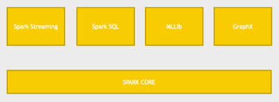
Fig: Components of Spark

Spark has a lot of depth to it so while you could just program at the RDD level within Spark core there are also libraries built on top of Spark that are part of Spark itself, it just comes along as part of the package.

Spark Streaming: is one of them, where instead of just doing batch processing of data you can actually input data in real time. So imagine you have a fleet of web servers that are producing logs that data can be ingested as it’s being produced and then Spark can actually analyze it across some window of time and you can output the results of that analysis to a database or some NoSQL data store or whatever you need to do, all with a few lines of code and Spark streaming.

Spark SQL: It’s basically a SQL interface to Spark. So again if you’re familiar with SQL you can just write SQL Queries against your data using Spark SQL or you SQL like functions to transform your data sets in Spark. This is really the direction that Spark is going in right now a lot of the optimization work (Catalyst and Tungsten projects) is really focused on the Spark SQL interface namely DataSets and DataFrames on Spark and that allows us to do even more optimizations beyond the directed basically because it can do SQL optimizations on the queries that you’re actually running and henceforth it’s faster than spark-core (RDD).

MLLib: An entire library of machine learning and data mining tools that you can run on a data set that’s in Spark. It can be very, very challenging to try to think about how to break a machine learning problem like clustering or you know regression analysis into mappers and reducers. You don’t have to though because Spark’s MLLib will figure that out for you and you can just create very high level classes for extracting meaning from the data that you have.

GraphX:. That’s the graph in the terms of graph theory. So imagine for example you have a social network graph you know, a graph of friends of friends, and you want to analyze the properties of that graph and see who’s connected to who and what way and what are the shortest path and things like that. GraphX provides a very extensible way of doing that.

It’s very easy to use as well so very rich ecosystem surrounding Spark that lets you do a wide variety of tasks on big data across the cluster. And that’s why I find Spark so exciting.